Post processing
After the image has been pre-processed and now, with only one product in our hands (master light), it’s time for the last stage.
The post processing stage consists of five essentials steps which are:
Background extraction
Color calibration
Deconvolution
Histogram stretch
Starless image creation
Star reduction
Color editing
In this part, we’ll showcase in detail each step (and those in between) the process which turns an almost unrecognizable image into a beautiful one.
Background extraction
When stacking hundreds of light frames into a master light image, we have to remember that every one of them was captured through different sky conditions. These conditions can be moonlight, light pollution, and non uniform sky brightness in overall. This means that 99% of the time, our master light will end with gradients, which are often difficult to remove. The goal with background extraction is to clean the image from all gradients to end up with the optimal foundation to continue the processing.
For background extraction/gradient correction we use Graxpert, a free to use program that takes Pixinsight’s “DynamicBackgroundExtraction” to a more intuitive interface, that sometimes produces even better results.
The first step into Graxpert is to obviously, import the image. One great thing about Graxpert is that it can open .xsif files, which retain all the astrometric data that’s after used to color calibrate the image. Then, we click on “Create grid”. This will place numerous background samples across the image that will be used to determine the brightness of it in each sample area. Often times, we have to adjust the “Grid tolerance” parameter, depending of the type of target. For instance, on nebulas we tend to use smaller tolerance values because it’s more likely that the background will be dominated by faint nebulosity, which doesn’t make for background itself. On the other hand, higher tolerance values are used in galaxies as the background will be pitch black, unless there is IFN or something similar.
With all the samples placed, now we click on “Calculate background”. This will create a synthetic background model that’ll be used to substract the background, and that’s it.


Color calibration
The next stage involves using Pixinsight and it’s SpectroPhotometricColorCalibration module. The objetive when calibrating the colors, it as the name itself says: to equal the color channel levels. In the case of a color image sensor, and due to the bayer matrix filter usually the color that will dominate the image will be green. That’s because of the RGGB pattern that the vast majority of color sensors feature, making green (G) double as prominent than red (R) and blue (B).
Apart of equalizing the color channels, Pixinsight’s SpectroPhotometricColorCalibration can use the astrometric solution present in the .xsif file to assign each star it’s true color. See more about SPCC here.
So, after importing back the image from Graxpert, we open the SPCC module and with the preview function (Alt+N) we select a background area to assign to the “Region of Interest” section, below the “Background Neutralization”. Then we click on “From Preview”, and select the created background preview. This will give the module an idea of how bright the background is to further balance the image color wise.
In case of a narrowband image, it is important to check the “Narrowband filters mode” and write on each channel the bandwitdh admitted by each filter. In the case of ours, we fill those fields with 7nm each as we use the L-eXtreme filter by Optolong that allows 7 nanometers of light to pass through.
In the case of a broadband color image, we simply leave all as it is when starting the process, except from the background preview described earlier.
With all of that, we can apply the process and our image will be correctly color calibrated. It is important to now STF auto stretch with all the channels linked, as the color balance is correct now.

Deconvolution
Time for the most feared process in Pixinsight: deconvolution.
But first, let us explain what deconvolution is. Deconvolution is the process of restoring an image whose light passed through the atmosphere essentially blurring it due to diffraction. Although, it is still considered sharpening, it’s a special kind of one as it utilizes the “point spread function” (PSF) to undo the effects of the atmosphere.
Now, here comes the part that would explain every single step to deconvolution, but the truth is that we no longer do it manually. Instead, we use the BlurXTerminator module made by Russel Croman, that works with AI to deliver the best deconvolution possible. But even this semi automated process requires some steps before it.
First, with the preview function we select a central area of the image, where the stars will be the most accurate in terms of how the atmosphere affected the image, and because it’s the area where the least optical aberrations will be visible, such as backfocus and coma that are typically accentuated at the corners. Then, we go to Script -> Render -> PSFImage. Note that this script is only available as a separate download from Hartmut Bornemann’s repository. With the preview selected and the script ready, we click on “Evaluate” and wait to the stars to be analyzed. After that and with the synthetic PSF image created, we’ll focus on two values: FWHMx and FWHMy. With those values, we can calculate the mid point between the two and with that, we can give BlurXTerminator the most accurate way of applying the process.
Later, in BlurXTerminator we uncheck the “Automatic PSF” box and check the “Correct First” one. Then, we fill the “PSF Diameter” with the resulting value of the “PSFImage” that we calculated earlier and with that, apply the process.


Histogram stretch
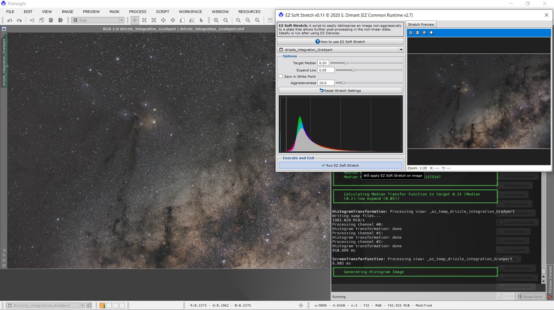
Once deconvolution is done, it is time to stretch the image. See, when opening an integrated master light image for the first time in Pixinsight, you will see that is completely black apart of some bright stars. That’s because we’re still in the linear stages, when all the data that was captured is still in the shadows region of the histogram. This is not a problem in the beginning, because some processes like background extraction, color calibration and deconvolution need to be applied in the linear stages. But past that, we need to bring those shadows up to the midtones areas, so that when we save our image, it won’t come dark. This is called stretching, as we are “stretching” the histogram graph.
For this step, we use Dark Archon’s EZ Processing Suite, as it offers an easy and efficient way to stretch our image. It is as simple as going to Script -> EZ Processing Suite -> EZ Soft Stretch. Default values will work very well most of the times, so the only step is to click on the “Run EZ Soft Stretch” button and you’ll now have a non-linear image.
Star reduction
After stretching and with the image now in a non-linear stage, we can continue with the star reduction step. This, in theory is not a mandatory step because it depends on if the image really need the stars to be reduced (for instance, we don’t necessarily need to reduce stars on star cluster images), but most of the time, the results will be beneficial. For this though, we need to substract the stars to create a “starless” image, as it is required by the star reduction script that we’re going to use. For star removal, we typically use the StarXTerminator process, developed once again by Russell Croman. After removing the stars, you can optionally work with the starless image on adjusting the contrast and levels.
Once you are done with the editing on the starless image, it’s time for merging the stars back in. For this, we’ll use a simple formula in the PixelMath process. The formula as it follows is “starless + star_mask”. For the star reduction itself, we always use Bill Blanshan’s star reduction PixelMath scripts. They work very well on all it’s presets and It’s up to the user taste on which to apply. Note that this script is dependent on the starless image generated earlier to work.


Color editing
For the final step, we will move to Adobe Photoshop. Here, we’ll open the image as a 16 bits TIFF (it needs to be outputted as that from Pixinsight) and begin to apply some curve adjustments. If you have a fairly recent version of PS, we recommend that you use the CameraRAW module, as it has multiple color editing options, including a selective color tool (color mixer). The goal with this step is to tweak color hues, increase or lower saturation and each color luminance. This section is an image enhancing step that depends only on the user’s taste.
The final step to all postprocessing is to export as a .jpeg and it’ll be ready to share!